728x90
Chapter 03에서는 '회귀 알고리즘과 모델 규제'에 대해 나온다.
소제목으로 '농어의 무게를 예측하라!' 라고 되어 있다.
드디어 분류가 아니라 예측을 향해 나아간다.
이 책에서는 농어의 data가 있는 상황에서 새로운 농어에 대해 길이 값만 가지고 있다.
기존 농어의 길이/무게 data들을 가지고 있을 때 새로운 농어의 무게를 예측해보자.
우선 기존 data의 산점도를 보자
##데이터 준비

import numpy as np

perch_length = np.array(
    [8.4, 13.7, 15.0, 16.2, 17.4, 18.0, 18.7, 19.0, 19.6, 20.0,
     21.0, 21.0, 21.0, 21.3, 22.0, 22.0, 22.0, 22.0, 22.0, 22.5,
     22.5, 22.7, 23.0, 23.5, 24.0, 24.0, 24.6, 25.0, 25.6, 26.5,
     27.3, 27.5, 27.5, 27.5, 28.0, 28.7, 30.0, 32.8, 34.5, 35.0,
     36.5, 36.0, 37.0, 37.0, 39.0, 39.0, 39.0, 40.0, 40.0, 40.0,
     40.0, 42.0, 43.0, 43.0, 43.5, 44.0]
     )
perch_weight = np.array(
    [5.9, 32.0, 40.0, 51.5, 70.0, 100.0, 78.0, 80.0, 85.0, 85.0,
     110.0, 115.0, 125.0, 130.0, 120.0, 120.0, 130.0, 135.0, 110.0,
     130.0, 150.0, 145.0, 150.0, 170.0, 225.0, 145.0, 188.0, 180.0,
     197.0, 218.0, 300.0, 260.0, 265.0, 250.0, 250.0, 300.0, 320.0,
     514.0, 556.0, 840.0, 685.0, 700.0, 700.0, 690.0, 900.0, 650.0,
     820.0, 850.0, 900.0, 1015.0, 820.0, 1100.0, 1000.0, 1100.0,
     1000.0, 1000.0]
     )

import matplotlib.pyplot as plt
plt.scatter(perch_length, perch_weight)
plt.xlabel('length')
plt.ylabel('weight')
plt.show()
from sklearn.model_selection import train_test_split

##train_test_split : train/test set 생성
train_input, test_input, train_target, test_target = train_test_split(
    perch_length, perch_weight, random_state=42)
print(train_input.shape, test_input.shape)
test_array = np.array([1,2,3,4])
print(test_array.shape)
test_array = test_array.reshape(2, 2)
print(test_array.shape)

train_input = train_input.reshape(-1, 1)
test_input = test_input.reshape(-1, 1)
print(train_input.shape, test_input.shape)
(42,) (14,)
(4,) (2, 2)
(42, 1) (14, 1)
결정 계수 (R^2)
분류를 할 때는 얼마나 정확하게 분류한 지 점수로 평가가 가능
예측 모델에서는 결정계수를 사용
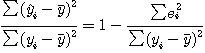
R^2 = 1 - (sum((타깃-예측)^2)) / (sum((타깃-평균)^2))
from sklearn.neighbors import KNeighborsRegressor
knr = KNeighborsRegressor()
# k-최근접 이웃 회귀 모델을 훈련합니다
knr.fit(train_input, train_target)

knr.score(test_input, test_target)
0.992809406101064
mean_absolute_error : 타깃과 예측의 절댓값 오차의 평균
from sklearn.metrics import mean_absolute_error
# 테스트 세트에 대한 예측을 만듭니다
test_prediction = knr.predict(test_input)
# 테스트 세트에 대한 평균 절댓값 오차를 계산합니다
mae = mean_absolute_error(test_target, test_prediction)
print(mae)
19.157142857142862
평균적으로 무게에 대한 예측 값과 실제 값이 19g정도 차이 난다는 결과
과대적합 vs 과소적합
과대적합(overfitting) : 훈련 세트만 점수가 좋고 테스트 세트에서 점수가 낮음
과소적합(underfitting) : 훈련세트보다 테스트세트의 점수가 더 높거나, 둘다 낮은 경우
print(knr.score(train_input, train_target))0.9698823289099254
knr.score(test_input, test_target) : 0.99
knr.score(train_input, train_target) : 0.96
훈련세트보다 테스트세트의 점수가 높으니 과소적합
# 이웃의 갯수를 3으로 설정
knr.n_neighbors = 3
# 모델을 다시 훈련
knr.fit(train_input, train_target)
print(knr.score(train_input, train_target))
0.9804899950518966
점수가 조금 더 올라 갔다
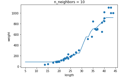
이웃 수를 변경하면서 결과를 확인해보자
# k-최근접 이웃 회귀 객체를 만듭니다
knr = KNeighborsRegressor()
# 5에서 45까지 x 좌표를 만듭니다
x = np.arange(5, 45).reshape(-1, 1)

# n = 1, 5, 10일 때 예측 결과를 그래프로 그립니다.
for n in [1, 5, 10]:
    # 모델 훈련
    knr.n_neighbors = n
    knr.fit(train_input, train_target)
    # 지정한 범위 x에 대한 예측 구하기
    prediction = knr.predict(x)
    # 훈련 세트와 예측 결과 그래프 그리기
    plt.scatter(train_input, train_target)
    plt.plot(x, prediction)
    plt.title('n_neighbors = {}'.format(n))
    plt.xlabel('length')
    plt.ylabel('weight')
    plt.show()
    print(knr.score(train_input, train_target))

728x90
'Programming > Machine Learning' 카테고리의 다른 글
| [혼공머신] 용어 03장 (0) | 2022.02.03 |
|---|---|
| [혼공머신] 04-1 로지스틱 회귀 (0) | 2022.01.23 |
| [혼공머신] 03-3 특성공학과 규제 (0) | 2022.01.22 |
| [혼공머신] 03-2 선형 회귀 (0) | 2022.01.16 |
| [혼공머신] 용어 02장 (0) | 2022.01.16 |
| [혼공머신] 02-2 데이터 전처리(data preprocessing) (0) | 2022.01.08 |
| [혼공머신] 용어 01장 (0) | 2022.01.05 |
| [혼공머신] 02-1 훈련세트와 테스트 세트 (0) | 2022.01.03 |
| [혼공머신] 01-3 마켓과 머신러닝 (0) | 2022.01.02 |
| Google Colaboratory (0) | 2022.01.01 |